Python Machine Learning

Step 1: Choosing features

The first step to a good machine learning model is always to choose the right features for your predictions. My original intentions had been to select a mix of both social and economic indicators and compare their relative accuracy in predicting birth rates/marriages, and also to combine some of these factors to obtain socio-economic indicators.

For Singapore data, a few of the sites that I consulted are:

Data.gov: ended up being my only source of data
Singstat: datasets tended to be too small
LTA Data Mall: I was impressed by the amount of data, but not relevant
Many other open source data on Singapore that was sadly irrelevant

A big drawback for me was that I could not find any datasets on social indicators that went far enough back (at least 1995) for me to have a sizeable dataset. While kind of comprehensive, the data on data.gov was also lacking in data with causal relationships, making it difficult to explore predictive models using the available data.

In the end, I settled with what I had (for now):

X data:

Year (I was expecting this to be a problem due to correlation issues)
Consumer Price Index, Monthly
Gross Domestic Product at Current Market Prices, Annually
Job Vacancy Rate, Quarterly
Resident Unemployment Rate, Quarterly
Average Weekly Paid Overtime Hours per Employee, Quarterly

Y data

Crude Birth Rates, Annually
Marriages under the Womens' Charter, Annually
Total Fertility Rate, Annually (I actually made a huge mistake and mixed up birth rates and TFR, so I had to redo some of my training)

All the data was obtained from data.gov in csv file format.

Step 2: Cleaning the Data

Cleaning the data proved to be more problematic than I thought it would be. Since the predicted values are annual data, I decided to process the quarterly and monthly data to return annual figures of [mean, standard deviation, direction, correlation]. "Direction" and "Correlation" will be elaborated on more later.

I used the pandas dataframe for data processing. It was a pain to pick up, but ultimately useful as it is an organised way to handle data that can be extended to large datasets, and has many built-in functions that make data processing not that difficult (e.g. iterrows, df.loc, df.apply). Pandas dataframes are also a well-supported type in python, and is handled with no problem by scikit-learn.

The processing steps were:

1. Split up the monthly and quarterly date data
Date data was split from "YYYY-month" or "YYYY-quarter" into "YYYY", then subsequent columns for each sub-division. This makes processing later on much easier as data from each subdivision are later handled as features of that year.

2. Handle empty values
Empty values are usually handled later on with the rest of the feature processing steps, but I had to handle them now as I was planning to use linear regression to obtain more features from sub-divided years, and linear regression cannot handle null values. Null values were simply replaced with the mean of the other values in the column.

3. Perform linear regression
Let linear regression be y = Ax+b. In this case, the y values are the quarterly or monthly data in each year, the x value is the sub-division of the y data in the year (ranging from 0 to 1). A linear regression is performed on each year and the "Direction" feature refers to the variable A in (y=Ax+b), while the feature "correlation" refers to the coefficient of determination, giving the strength of the linear relationship between x and y. The linear regression was performed using sklearn LinearRegression method.

After going in to do some simple data procesing myself (deleting columns etc.), the data is now ready for further processing.

Step 3: Data Exploration

Now that the data has been prettified, it is time for some visualisation to gain insights on the data on hand. From here on, I will foxus on total Fertility rate as the predicted y value.

First, I combined all the features into one large features dataframe. I was initially considering adding polynomial features and performing PCA to narrow down the feature space, but after performing train-test split, my number of data points and number of features became comparable and I did not want to risk having too many features.

Next, I looked at the correlations between the y data and each of the features. By using the pandas .coor() function, I obtained a list of correlations.

python3 regression_methods.py
value            1.000000
overtime_mean    0.854868
jobvac_mean      0.776832
jobvac_std       0.736551
jobvac_corr      0.624030
overtime_std     0.567258
cpi_corr         0.464942
unemp_dir        0.249930
labcost_dir      0.120821
labcost_corr     0.029503
unemp_std        0.014350
labcost_std     -0.076240
cpi_dir         -0.132496
unemp_corr      -0.192243
overtime_corr   -0.243318
cpi_std         -0.272496
labcost_mean    -0.414698
overtime_dir    -0.427331
unemp_mean      -0.523999
jobvac_dir      -0.724803
cpi_mean        -0.767823
gdp_value       -0.827605
year            -0.918486
Name: value, dtype: float64

Here you can see that "year" is most highly correlated with the TFR, which may present as a problem by creating a model that suggests that Singapore's falling birth rate is inevitable. "Overtime_mean" is also highly correlated with TFR, however there is the problem of correlation vs. causation, and the causal effect between these two variables is unclear.

To gain greater insights, I picked 6 of the features most linearly correlated with total fertility rates and plotted them all against each other in a scatter plot:

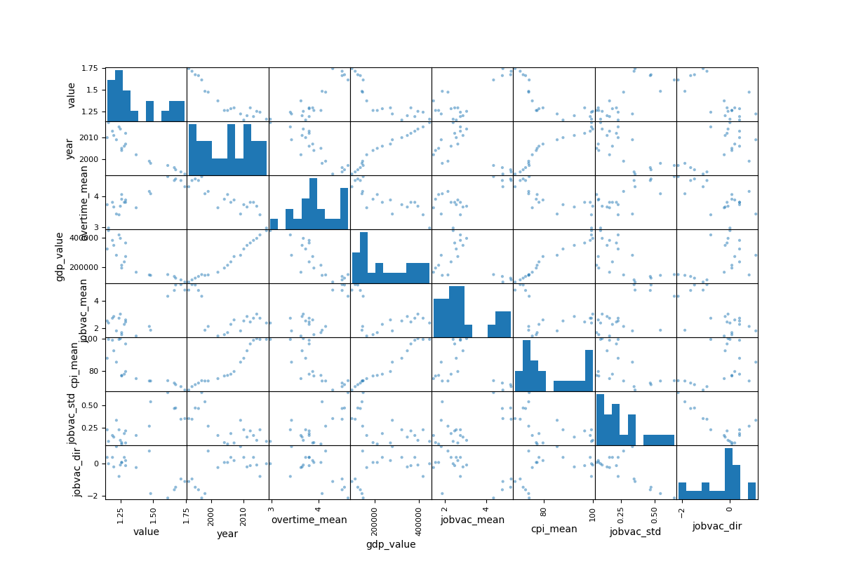
From the scatter plot we can see that the relationship between "year" and TFR more closely follows an exponential function, as well as with other factors "gdp_value" and "cpi_mean". Thus, I performed an exponential decay function on these three features to hopefully give a better linear correlation between the features and the y value.

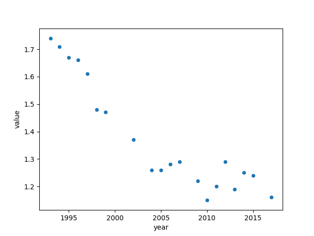
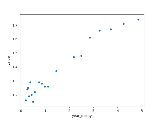
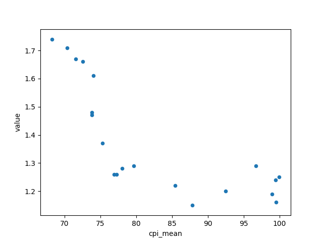
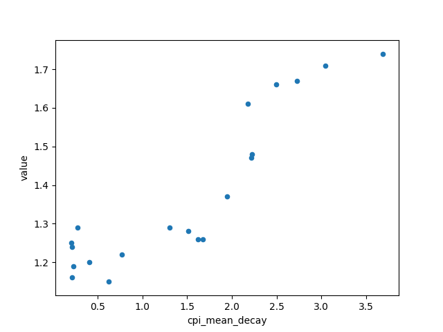
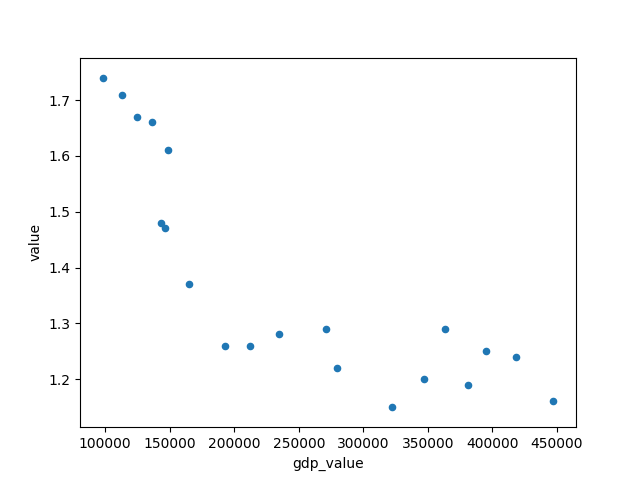
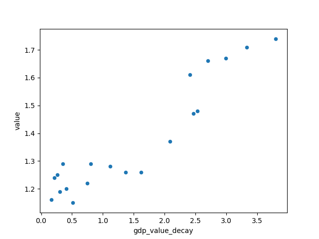
After fitting the exponential function, the improvement looks marginal in the scatter plot, but the correlation values showed a small improvement and I decided to just take what I have and move on to the transformation pipeline.

python3 regression_methods.py
Correlation matrix for decay features:
value              1.000000
year_decay         0.975068
gdp_value_decay    0.937049
cpi_mean_decay     0.904391
overtime_mean      0.854868
jobvac_mean        0.776832
jobvac_std         0.736551
jobvac_corr        0.624030
overtime_std       0.567258
cpi_corr           0.464942
unemp_dir          0.249930
labcost_dir        0.120821
labcost_corr       0.029503
unemp_std          0.014350
labcost_std       -0.076240
cpi_dir           -0.132496
unemp_corr        -0.192243
overtime_corr     -0.243318
cpi_std           -0.272496
labcost_mean      -0.414698
overtime_dir      -0.427331
unemp_mean        -0.523999
jobvac_dir        -0.724803
cpi_mean          -0.767823
gdp_value         -0.827605
year              -0.918486
Name: value, dtype: float64

Step 4: Pipeline

A pipeline is a series of transformers applied to the data before it is used for training a model. Each transformer has a fit() and transform() function (as explained in SKLearn Tips and Tricks) and are applied sequentially on the data fed into the pipeline. For processing the data for a regression model, my sklearn pipeline consists of the SimpleImputer and StandardScaler.

The SimpleImputer is a transformer provided by sklearn that helps to fill in null values. By specifying the strategy as "mean", I am filling in the null values with the mean of all the other values in the column. However, much of the null values in the data have already been handled in an earlier part to obtain additional features through linear regression, thus the Imputer here is for additional checking for null values, and to process future data. The StandardScaler scales the data to a certain mean and range. Of the two available strategies, standard-deviation and min-max, I chose to implement the stndard-deviation strategy as it is less affected by outliers.

Step 5: Testing Regression Methods

After preparing the data for the various sklearn regressions, it is now easy to test out the data on multiple kinds of regression models. The few that I have chosen are: linear regression, decision tree regressor, random forest regressor and SVM regressor (with linear, poly, rbf and sigmoid kernels). I decided against a polynomial regression as the large number of features will make the number of combinations expand very rapidly, and my data set will become much smaller than the number of features (resulting in the curse of dimentionality).

After training the training data using the models stated above, I evaluated the error of the models on the training data itself:

python3 -c 'import regression_methods; InitialRegression(training_set_err)'
Error on training set for linear regression: 2.764433037591714e-16
Error on training set for decision tree regressor: 0.0
Error on training set for random forest regressor: 0.02825774230188955
python3 -c 'import regression_methods;InitialRegressionSVM(training_set_err)'
Error on training set for SVM linear regression: 0.07440866416057071
Error on training set for SVM poly regression: 0.07199860703890534
Error on training set for SVM rbf regression: 0.08604743906320432
Error on training set for SVM sigmoid regression: 0.07307290024471638

It can be seen that the linear regression and decision tree regressor appear to overfit the training data quite badly, resulting in an extremely small error. Further evaluation of the models are done with a Leave-One-Out cross validation test (a comparison of LOOC and K-Fold CV can be found on the Machine Learning Tips page) and errors are as shown:

python3 -c 'import regression_methods; InitialRegression(cross_validation_err)'
Cross Validation error for linear regression:
Scores:  [0.054842   0.00399597 0.03568356 0.13978444 0.04281256 0.04604125 0.05829293
 0.07240102 0.01860834 0.00776581 0.01481755 0.00364524 0.05873764 0.02579565 0.09859207
 0.15252078 0.07862143 0.00330323 0.07660888 0.53208627]
Mean:  0.07624783154544243
Standard deviation:  0.11248767941765023

Cross Validation error for decision tree regressor:
Scores:  [0.21 0.08 0.05 0.14 0.1  0.   0.1  0.01 0.18 0.06 0.06 0.06 0.04 0.03 0.04 0.19
 0.1  0.06 0.05 0.11]
Mean:  0.0835
Standard deviation:  0.05694514904713128

Cross Validation error for random forest regressor:
Scores:  [0.111 0.109 0.08  0.02  0.035 0.03  0.067 0.054 0.035 0.073 0.053 0.001 0.064
 0.114 0.089 0.005 0.036 0.02  0.024 0.044]
Mean:  0.05319999999999999
Standard deviation:  0.0335687354542884

python3 -c 'import regression_methods;InitialRegressionSVM(training_set_err)'
Cross Validation error for SVM linear regression:
Scores:  [0.09080374 0.11937214 0.07250952 0.02995561 0.1213769  0.07664682 0.01063642
 0.0770035  0.11281128 0.12311391 0.0753716  0.05734756 0.15617136 0.05845668 0.01405324
 0.06087444 0.03156834 0.08382428 0.0609033  0.05759235]
Mean:  0.07451965069118438
Standard deviation:  0.03731505145643753

Cross Validation error for SVM poly regression:
Scores:  [0.0639619  0.08832214 0.06911489 0.00294872 0.14626911 0.06799292 0.01059334
 0.14858441 0.22023286 0.16793713 0.07181147 0.04379031 0.17939204 0.04106339 0.01160151
 0.14913094 0.0542449  0.04976189 0.07783498 0.05844717]
Mean:  0.0861518011138705
Standard deviation:  0.059731644134825415

Cross Validation error for SVM rbf regression:
Scores:  [0.09845441 0.18313329 0.10534654 0.07050253 0.15375965 0.09234144 0.05357059
 0.10884812 0.13208508 0.10881556 0.18629143 0.07108267 0.18490334 0.19231357 0.00442793
 0.07041296 0.01779497 0.08402715 0.10365277 0.08741709]
Mean:  0.10545905412234675
Standard deviation:  0.05230333381419113

Cross Validation error for SVM sigmoid regression:
Scores:  [0.10538674 0.10699255 0.06575242 0.01325729 0.10146539 0.07935778 0.01314629
 0.04998052 0.08224383 0.11372819 0.0610924  0.05436151 0.14048255 0.07774499 0.01526464
 0.04585146 0.00466904 0.0826025 0.06211805 0.08907408]
Mean:  0.0682286110514455
Standard deviation:  0.03629890887323988

It can be seen that the error on the cross validation test for the linear regression and decision tree regressor is much larger (of multiple orders of magnitude) than the error on the whole training set, showing that the linear regression and decision tree regressor has indeed badly overfitted the training data.

After performing the training and cross validation for each regression method, I decided to go with the Random Forest Regressor (CV error: 0.0531±0.0335) as top choice and the SVM sigmoid regression (CV error: 0.0682±0.0362) as second choice for proceeding with the fine-tuning of the models.

Step 6: Hypertuning Random Forest Regression

After choosing the best performing model, I went on to hypertune the free parameters of the model. From the random forest regressor documentation in sklearn, the important features appear to be:

n_estimators: No. of decision trees in the forest
max_depth: Maximum depth of a tree
min_samples_split: Minimum number of samples required to split an internal node
min_samples_leaf: Minimum number of samples required to form a leaf
max_features: No. of features (relative to all the features) to consider when choosing the best split
bootstrap: Whether bootstrap samples are used when building trees

I first performed a random search through multiple test values for each parameter to narrow down the range of values to be tested in detail later on, so as to reduce the time needed for training. At this stage, if a lot of combinations are being tested, it is useful to set the search to "verbose" to track the progress of the search.

After obtaining the best params from the random search, I then performed a grid search to systematically obtain the best combination of parameters to optimise the cross validation score. Note that the nmber of combinations to search are multipled for each parameter, so n_combinations = n_1 * n_2 * n_3 * ... * n_x, where n refers to the number of values tested for each parameter for x parameters. A "verbose" setting is also useful here to ensure that the search is proceeding correctly.

The best parameters obtained from the grid search are shown below, as well as the improvement in model performance (base model is the random forest regression conducted with default parameters). The hypertuning only yielded an improvement in performance of 0.92%, showing that hypertuning does not significantly improve the accuracy of the model. Instead, other factors like feature selection and processing and amount of data may play a larger role in improving the model.

python3 -c 'import regression_methods; evaluateTest(rf_grid_best_params)'
best params: {'max_depth': 110, 'max_features': 'sqrt', 'n_estimators': 30, 'min_samples_split': 7, 'bootstrap': True, 'min_samples_leaf': 1}

Model Performance (base model)
Average Error: 1.4406
Accuracy = 86.34%

Model Performance (best model)
Average Error: 1.3449
Accuracy = 87.26%

Next part.

python3 anaylse.py
best params: {'max_depth': 110, 'max_features': 'sqrt', 'n_estimators': 30, 'min_samples_split': 7, 'bootstrap': True, 'min_samples_leaf': 1}

Model Performance
Average Error: 0.2073
Accuracy = 94.74%

Learning Curve (Random Forest Regressor)